CCN 2023 | Tutorial - Analyzing and comparing deep neural networks

Summary

Deep networks are considered to be black boxes because we cannot answer fundamental questions about their inner workings. In this part of the tutorial, we will show how to measure the dimensionality of representations and weights of deep networks. We will also compare networks trained from different initializations to assess the similarity of their representations and weights.

Run this notebook interactively!

Here’s a link to this notebook on Google Colab.

Experimental setup

Install all required dependencies

%pip install git+https://github.com/BonnerLab/ccn-tutorial.git

Load modules and functions

import time
from tqdm.notebook import tqdm
import copy

import torch
from torch import nn
import torch.utils.data.dataset
import torchvision.transforms as transforms
import torchvision.datasets as datasets

import numpy as np
from matplotlib import pyplot as plt

Define various helper functions

DEVICE = torch.device("cuda" if torch.cuda.is_available() else "cpu")


def get_datasets():
    """Returns train and validation datasets."""
    mean = [0.485, 0.456, 0.406]
    std = [0.229, 0.224, 0.225]
    data_transforms = [
        transforms.ToTensor(),
        transforms.Normalize(mean=mean, std=std),
        transforms.Grayscale(),
    ]

    dataset_class = datasets.CIFAR10

    def get_dataset(train: bool):  # Returns the train or validation dataset.
        root = "./data"
        kwargs = dict(
            root=root,
            transform=transforms.Compose(data_transforms),
            train=train,
            download=True,
        )
        dataset = dataset_class(**kwargs)
        return dataset

    train_dataset = get_dataset(train=True)
    val_dataset = get_dataset(train=False)
    return train_dataset, val_dataset


def get_dataloaders(batch_size):
    """Returns train and validation dataloaders."""
    train_dataset, val_dataset = get_datasets()

    def get_dataloader(dataset, shuffle):
        return torch.utils.data.DataLoader(
            dataset,
            batch_size=batch_size,
            shuffle=shuffle,
            num_workers=0,
            pin_memory=True,
        )

    train_loader = get_dataloader(train_dataset, shuffle=True)
    val_loader = get_dataloader(val_dataset, shuffle=False)
    return train_loader, val_loader


def initialize_mlp_model(dims):
    """Create a simple MLP model.
    :param dims: list of dimensions of each layer, should begin with dimension of input and end with number of classes.
    :return: Sequential MLP model
    """
    layers = [torch.nn.Flatten()]
    for i in range(len(dims) - 1):
        layers.append(nn.Linear(dims[i], dims[i + 1], bias=False))
        if i < len(dims) - 2:
            layers.append(nn.ReLU())
    model = nn.Sequential(*layers)
    return model


def initialize_cnn_model(
    channels, spatial_size=32, kernel_size=5, stride=2, num_classes=10
):
    """Create a simple CNN model.
    :param channels: list of channels of each convolutional layer, should begin with number of channels of input.
    :return Sequential CNN model
    """
    layers = []
    for i in range(len(channels) - 1):
        layers.append(
            nn.Conv2d(channels[i], channels[i + 1], kernel_size=5, stride=2, bias=False)
        )
        spatial_size = ceil_div(spatial_size - kernel_size + 1, stride)
        layers.append(nn.ReLU())

    layers.extend(
        [
            nn.Flatten(),
            nn.Linear(channels[-1] * spatial_size**2, num_classes, bias=False),
        ]
    )
    model = nn.Sequential(*layers)
    return model


def ceil_div(a: int, b: int) -> int:
    """Return ceil(a / b)."""
    return a // b + (a % b > 0)


def train_model(model, train_loader, val_loader, lr=0.01, momentum=0.9, num_epochs=5):
    """Simple training of a model with SGD."""
    optimizer = torch.optim.SGD(model.parameters(), lr=lr, momentum=momentum)
    loss_fn = nn.CrossEntropyLoss()

    epoch = 0
    model.to(DEVICE)
    while True:
        # Evaluate on validation set.
        one_epoch(
            loader=val_loader,
            model=model,
            loss_fn=loss_fn,
            optimizer=optimizer,
            epoch=epoch,
            is_training=False,
        )

        # Stop if we are at the last epoch.
        if epoch == num_epochs:
            break

        # Train for one epoch (now epoch counts the current training epoch).
        epoch += 1
        one_epoch(
            loader=train_loader,
            model=model,
            loss_fn=loss_fn,
            optimizer=optimizer,
            epoch=epoch,
            is_training=True,
        )

    # Ensure evaluation mode and disable gradients before returning trained model.
    model.eval()
    for param in model.parameters():
        param.requires_grad = False
    return model


def one_epoch(loader, model, loss_fn, optimizer, epoch, is_training):
    """Run one train or validation epoch on the model.
    :param loader: dataloader to use
    :param model: model to train or evaluate
    :param loss_fn: loss function (not used during evaluation)
    :param optimizer: optimizer (not used during evaluation)
    :param epoch: current epoch number (for tqdm description)
    :param is_training: whether to train the model or simply evaluate it
    :return: average accuracy during the epoch
    """
    name_epoch = "Train" if is_training else "Val"
    name_epoch = f"{name_epoch} epoch {epoch}"
    accuracy_meter = AverageMeter()

    if is_training:
        model.train()
    else:
        model.eval()

    with torch.set_grad_enabled(is_training):
        it = tqdm(loader, desc=name_epoch)
        for x, y in it:
            x = x.to(DEVICE, non_blocking=True)
            y = y.to(DEVICE, non_blocking=True)
            y_hat = model(x)

            loss = loss_fn(y_hat, y)
            accuracy = 100 * torch.sum((y_hat.argmax(-1) == y).float())
            accuracy_meter.update(val=accuracy.item(), n=y.shape[0])
            it.desc = f"{name_epoch}: {accuracy_meter.avg():.2f}% accuracy"

            if is_training:
                # compute gradient and do SGD step
                optimizer.zero_grad()
                loss.backward()
                optimizer.step()

    return accuracy_meter.avg()


class AverageMeter(object):
    """Computes and stores the average and current value."""

    def __init__(self):
        self.sum = 0
        self.count = 0

    def update(self, val, n):
        self.sum += val
        self.count += n

    def avg(self):
        return self.sum / self.count


def get_activations(x, layers, model):
    """Returns the hidden activations of a model.
    :param x: input to use, tensor of shape (B, C, [N, N])
    :param layers: list of integers (j corresponds to output of j-th layer, 0 corresponds to input of model)
    :param model: model to use (should be Sequential)
    :return: list of saved activations of same length as layers
    """
    saved_activations = []

    def hook(self, inputs, output):  # inputs is a tuple, we assume it is of length 1
        saved_activations.append(inputs[0])

    # Register hooks to save activations of chosen layers.
    for layer in layers:
        model[layer].register_forward_hook(hook)

    # Forward of model: hooks will be run and activations will be saved.
    _ = model(x)

    # Clear hooks.
    for layer in layers:
        model[layer]._forward_hooks.clear()

    return saved_activations


def compute_activation_covariances(loader, layers, model1, model2=None):
    """Compute the (cross-)covariance of hidden activations at several layers of one or two models.
    :param loader: data loader to use
    :param layers: list of integers (j corresponds to output of j-th layer, 0 corresponds to input of model)
    :param model1: model to use (should be Sequential)
    :param model2: optional model for a cross-covariance (if None, compute the self-covariance of model1)
    :return: list of computed covariances (C1, C2), of same length as layers
    """
    meters = [AverageMeter() for _ in layers]

    # Version of get_activations which treats spatial dimensions as additional batch dimensions.
    get_acts = lambda *args: [space_to_batch(act) for act in get_activations(*args)]

    for x, _ in tqdm(loader, desc="Computing activation covariance"):
        x = x.to(DEVICE)
        activations1 = get_acts(x, layers, model1)
        activations2 = activations1 if model2 is None else get_acts(x, layers, model2)

        for i, (act1, act2) in enumerate(zip(activations1, activations2)):
            cov = act1.T @ act2  # (C1, C2), sum of outer products over the batch
            meters[i].update(val=cov, n=act1.shape[0])

    return [meter.avg() for meter in meters]


def space_to_batch(x):
    """(B, C, [M, N]) to (B[MN], C)."""
    if x.ndim == 4:
        x = x.permute(0, 2, 3, 1)  # (B, M, N, C)
        x = x.reshape((-1, x.shape[-1]))  # (BMN, C)
    return x


def clip(model, layer, basis, dimensions, loader):
    """Clip and evaluate a model.
    :param model: trained model to clip (should be Sequential)
    :param layer: index of layer to clip
    :param basis: ordered orthogonal basis vectors for the clipping, of shape (num_vectors, input_dim)
    :param dimensions: list of clipping dimensions
    :param loader: data loader to use for the evaluation
    :return: list of accuracies
    """
    models = []
    for dim in dimensions:
        projector = basis[:dim].T @ basis[:dim]
        model_clipped = copy.deepcopy(model)
        model_clipped[layer].weight = torch.nn.Parameter(
            model_clipped[layer].weight @ projector, requires_grad=False
        )
        models.append(model_clipped)

    return evaluate(models, loader, desc="Evaluation after clipping")


def evaluate(models, loader, desc="Evaluation"):
    """Evaluate a list of models.
    :param models: list of models to evaluate
    :param loader: dataloader to use for evaluation
    :return: list of accuracies, one per model
    """
    accuracy_meters = [AverageMeter() for _ in models]

    it = tqdm(loader, desc=desc)
    for x, y in it:
        x = x.to(DEVICE, non_blocking=True)
        y = y.to(DEVICE, non_blocking=True)
        for model, accuracy_meter in zip(models, accuracy_meters):
            y_hat = model(x)
            accuracy = 100 * torch.sum((y_hat.argmax(-1) == y).float())
            accuracy_meter.update(val=accuracy.item(), n=y.shape[0])

    return [accuracy_meter.avg() for accuracy_meter in accuracy_meters]


def generate_network(reference_model, state_dict_keys, train_loader, val_loader):
    """Generate a new network with a similar performance from a reference network.
    NOTE: this function does not take care of batch norm parameters.
    They should be recomputed when the previous layer has been generated.
    NOTE: this function can be extended in many ways: sample only a subset of layers, change the width of some layers,
    use weight covariances averaged over several models...
    :param reference_model: reference model for the rainbow model
    :param state_dict_keys: list of keys in model state dict to sample
    :param train_loader: dataloader used for computing alignment between reference and generated model
    :param val_loader: dataloader used to evaluate performance of generated model
    :return: list of accuracies, corresponding to the reference and generated models
    """
    # The generated model is initialized as a copy of the reference model.
    generated_model = copy.deepcopy(reference_model)
    state_dict = generated_model.state_dict()

    # At beginning of loop, this contains alignment at layer j between generated model and reference model
    # (used to determine the correct covariance to generate atoms at layer j).
    alignment = None  # alignment matrix (C_in_reference, C_in_generated)

    results = {}  # metric, layer_idx -> performance

    # Generate each layer iteratively.
    for j, key in enumerate(state_dict_keys):
        weight = state_dict[
            key
        ]  # (C_out, C_in, [h, w]) depending on conv or fully connected layer

        # Compute new weight in reference space.
        if j < len(state_dict_keys) - 1:
            # Sample Gaussian weights with the same covariance as the trained weights.
            # Compute square root of covariance with an SVD (more efficient when C_out << C_in*h*w).
            weight_flat = weight.reshape((weight.shape[0], -1))  # (C_out, C_in*h*w)
            u, s, vt = torch.linalg.svd(
                weight_flat, full_matrices=False
            )  # (C_out, R), (R,), (R, C_in*h*w) where R = rank
            white_gaussian = torch.randn(
                u.shape, dtype=weight.dtype, device=weight.device
            )  # (C_out, R)
            colored_gaussian = white_gaussian @ (s[:, None] * vt)  # (C_out, C_in*h*w)
            new_weight = colored_gaussian.reshape(weight.shape)  # (C_out, C_in, [h, w])
        else:
            # Use the trained classifier.
            new_weight = weight

        # Realign the weights from the reference model to the generated model (necessary after first layer).
        if j > 0:
            new_weight = contract(
                new_weight, alignment.T, axis=1
            )  # C_in_reference to C_in_generated

        # Set the new weights in the generated model.
        # NOTE: this an intermediate model, as sampling the j-th layer means that the j+1-th layer is no longer aligned.
        # As such, if evaluated as is, its accuracy would be that of a random guess.
        state_dict[key] = new_weight
        generated_model.load_state_dict(state_dict)

        # Then compute alignment of the generated network with the reference model for the next layer.
        if j < len(state_dict_keys) - 1:
            next_key = state_dict_keys[j + 1]
            # Compute index of layer by relying on Sequential naming convention: next_key is "{layer_idx}.weight".
            layer = int(next_key.split(".")[0])

            [activation_covariance] = compute_activation_covariances(
                train_loader, [layer], reference_model, generated_model
            )  # (C_in_reference, C_in_generated)

            u, s, vh = torch.linalg.svd(
                activation_covariance, full_matrices=False
            )  # (C_in_reference, R), (R,), (R, C_in_generated)
            alignment = u @ vh  # (C_in_reference, C_in_generated)

    # Evaluate models.
    return evaluate(
        [reference_model, generated_model], val_loader, desc="Evaluation after sampling"
    )


def contract(tensor, matrix, axis):
    """tensor is (..., D, ...), matrix is (P, D), returns (..., P, ...)."""
    t = torch.moveaxis(tensor, source=axis, destination=-1)  # (..., D)
    r = t @ matrix.T  # (..., P)
    return torch.moveaxis(r, source=-1, destination=axis)  # (..., P, ...)

Dataset

The CIFAR-10 dataset contains 50,000 training and 10,000 validation images of resolution 32 \times 32. They are divided in 10 classes:

The dataset is automatically downloaded and loaded in memory with torchvision (see the CIFAR10 class). Here we do not perform any data augmentation for simplicity, and convert the images to grayscale for computational efficiency.

Load the dataset

train_loader, val_loader = get_dataloaders(batch_size=128)
class_labels = [
    "airplane",
    "automobile",
    "bird",
    "cat",
    "deer",
    "dog",
    "frog",
    "horse",
    "ship",
    "truck",
]

# Draw one batch to show some training images
x, y = next(train_loader.__iter__())

fig, ax = plt.subplots(ncols=5, figsize=(10, 3))
fig.suptitle("Random images from the training set")
for i in range(5):
    ax[i].imshow(x[i].cpu().numpy().transpose(1, 2, 0), cmap="gray")
    ax[i].axis("off")
    ax[i].set_title(class_labels[y[i]])

Downloading https://www.cs.toronto.edu/~kriz/cifar-10-python.tar.gz to ./data/cifar-10-python.tar.gz
Extracting ./data/cifar-10-python.tar.gz to ./data
Files already downloaded and verified

Network architecture and training

We begin with a barebones feedforward network architecture with two hidden layers.

It computes the function f(x) = \theta \sigma(W_2 \sigma(W_1 x))

where:

x \in \mathbb R^d is an input image reshaped as a vector (d = 32 \times 32),
W_1 \in \mathbb R^{n_1 \times d} are the weights of the n_1 neurons in the first layer,
W_2 \in \mathbb R^{n_2 \times n_1} are the weights of the n_2 neurons in the second layer,
\theta \in \mathbb R^{c \times n_2} are the weights of the classifier, which predicts log-likelihoods for the c = 10 classes,
\sigma is a pointwise non-linearity (here a ReLU).

Initialize the model

dims = [  # sizes of layers
    32 * 32,  # input dim
    512,  # hidden dim
    256,  # hidden dim
    10,  # output dim (number of classes)
]
model = initialize_mlp_model(dims)
print(model)

Sequential(
  (0): Flatten(start_dim=1, end_dim=-1)
  (1): Linear(in_features=1024, out_features=512, bias=False)
  (2): ReLU()
  (3): Linear(in_features=512, out_features=256, bias=False)
  (4): ReLU()
  (5): Linear(in_features=256, out_features=10, bias=False)
)

We train the network for 5 epochs (passes over the training set). We measure the average accuracy (frequency at which the network correctly predicts the correct class). On a held-out validation set, it increases from 10%, which corresponds to a random guess, to about 43%.

Note: accuracies below 90% are generally considered low, with state-of-the-art networks reaching 99.5% accuracy. The accuracy can be increased by switching to a convolutional architecture (see below), increasing the width and depth of the network, adding data augmentation, training for a longer time, etc.

Train the model

_ = train_model(model, train_loader, val_loader, num_epochs=5)

Analyzing a trained network

Measuring the dimensionality of hidden representations

At each layer, we can measure the dimensionality of the corresponding hidden representation with a PCA. We thus compute the covariance of the representation. Let \varphi(x) denote the representation of the input x at the given layer. Then, we compute its covariance:

\mathbb E_x\left[\varphi(x) \, \varphi(x)^\top\right].

Note: We shall act as if the mean \mathbb E_x \left[ \varphi(x) \right] was zero for simplicity. Typically, this is enforced by a normalization layer such as batch normalization or layer normalization.

One might want to compute the hidden representations of all the training images:

\newcommand{\vertbar}{\rule[-1ex]{0.5pt}{2.5ex}} X = \left[ \begin{array}{cccc} \vertbar & \vertbar & & \vertbar \\ \varphi(x_1) & \varphi(x_2) & \cdots & \varphi(x_n) \\ \vertbar & \vertbar & & \vertbar \end{array} \right]^\top,

and compute the covariance with \frac{1}{n} X^\top X. However, this matrix is usually too big to fit into memory (especially for larger datasets)!

We thus adopt the approach of mini-batching. We break the dataset into batches (little chunks) and load it in memory one batch at a time. The covariance can then be computed iteratively in this way:

covariance_accumulator = 0
num_samples = 0
for x in dataloader:                   # x has shape (batch_size, input_dim)
    z = phi(x)                         # z has shape (batch_size, repr_dim)
    covariance_accumulator += z.T @ z  # shape (repr_dim, repr_dim)
    num_samples += z.shape[0]          # We have processed batch_size samples.
covariance = covariance_accumulator / num_samples

This “trick” works for the expected value of any function over the data. The mini-batching and loading into memory is taken care of by PyTorch’s DataLoader class. Note that contrary to model training, the batch size here does not affect the end result, it influences only the time and memory complexity of the computation. The batch size should be small enough to fit into memory, but as large as possible to exploit the parallelization of computation (as done automatically by PyTorch on a GPU backend).

Compute activation covariances

# Layers 3 and 5 correspond to the output of the two ReLUs.
layers = [3, 5]
activation_covariances = compute_activation_covariances(train_loader, layers, model)
# Activation covariances is a list of covariances, one per layer.

Once we have computed the covariance of the hidden representation, we can diagonalize it to compute its eigenvalues, which encode the variance along each principal component (we do not concern ourselves with cross-validation here).

As another way of evaluating the importance of each principal component, we can perform clipping. This consists of inserting an operation in the middle of the network, which projects the hidden representation on its first k principal components. We can then evaluate the accuracy of the network as a function of k, which allows measuring the cumulative “information” stored in the first k PCs.

Visualize activation covariance spectrum and the result of clipping

fig, ax = plt.subplots(figsize=(8, 8), nrows=2, ncols=2)

for layer_idx in range(2):
    activation_covariance = activation_covariances[layer_idx]
    activation_eigenvalues, activation_eigenvectors = torch.linalg.eigh(
        activation_covariance
    )
    # (num_eig,), descending order
    activation_eigenvalues = activation_eigenvalues.flip(-1)

    # (num_eig, dim), descending order
    activation_eigenvectors = activation_eigenvectors.flip(-1).T

    # Plot the eigenvalues of the activation covariances.
    plt.sca(ax[0][layer_idx])
    plt.title(f"Activation covariance spectrum (layer {layer_idx + 1})")
    y = activation_eigenvalues.cpu().numpy()
    x = 1 + np.arange(len(y))
    plt.plot(x, y, color="tab:green")
    plt.yscale("log")
    plt.xscale("log")
    plt.xlabel("Rank")
    plt.ylabel("Eigenvalue")

    # Clipping analysis.
    dimensions = 1 + np.arange(activation_eigenvectors.shape[1])
    accuracies = clip(
        model, 2 * layer_idx + 3, activation_eigenvectors, dimensions, val_loader
    )

    plt.sca(ax[1][layer_idx])
    plt.plot(dimensions, accuracies, color="tab:red")
    plt.title(f"Accuracy after activation clipping (layer {layer_idx + 1})")
    plt.xlabel("Maximum rank")
    plt.ylabel(r"Accuracy (%)")
    plt.xscale("log")

plt.tight_layout()
plt.show()

We see that the learned representations have a power law spectrum. Further, they can be somewhat reduced in dimension at little cost in accuracy (note that rank is in log scale).

Measuring the dimensionality of neuron weights

Let us focus on the first layer. The weight matrix W_1 of size n_1 \times d contains the weights of the n_1 neurons in the first layer, each being a d-dimensional vector. (This also applies to the other layers. For instance, the second weight matrix W_2 of size n_2 \times n_1 contains the weights of the n_2 neurons in the second layer, each being an n_1-dimensional vector.)

We can view these neurons as being samples from a continuous distribution, and then estimate statistical properties (moments) of this distribution. For instance, assuming a zero mean, we can compute the covariance of the neuron weights as: C = \frac{1}{n_1} W_1^\top W_1

The covariance reveals how the global geometry of the representation is modified by the neuron population. Indeed, the representation computed by the first layer is \varphi_1(x) = \sigma(W_1 x). Focusing on the weight matrix W_1, we can decompose its effect with a singular value decomposition: W_1 = U \Sigma V^\top.

Recall that the right singular vectors V are also the eigenvectors of the covariance C, while the singular values \Sigma are directly related to the eigenvalues of the covariance C.

This implies that the first layer \sigma(W_1 x) computes the following steps:

an orthogonal change of basis to the PCA basis of the neuron weights,
a scaling along each principal component (proportional to the square root of the covariance eigenvalues),
another orthogonal change of basis, which defines the basis in which the non-linearity \sigma is applied.

The covariance eigenvalues and eigenvectors thus define how the neural code globally changes the geometry of its input before the non-linearity. In particular, if the covariance is low-rank, it indicates that the representation only depends on a low-dimensional projection of the input.

To interpret the eigenvalues of the covariance, we can compare their values after training with their values at initialization. Neuron weights are initialized from a distribution with covariance identity (in PyTorch, each component is by default independently drawn from a uniform distribution). However, the eigenvalues of the empirical covariance computed from only the n_1 neurons are not all one but follow the Marchenko-Pastur distribution. This comparison allows estimating which eigenvalues are significantly non-random.

Visualize weight covariance spectrum and the result of clipping

fig, ax = plt.subplots(figsize=(8, 8), nrows=2, ncols=2)

for layer_idx in range(2):
    weight_matrix = model[2 * layer_idx + 1].weight  # (N, D)
    # Compute eigenvalues and eigenvectors of weight covariance efficiently from the SVD.
    _, weight_singular_values, weight_eigenvectors = torch.linalg.svd(
        weight_matrix, full_matrices=False
    )  # (num_eig, dim), descending order
    weight_eigenvalues = weight_singular_values**2 / weight_matrix.shape[0]

    # Compare with eigenvalues at initialization.
    init_weight_matrix = initialize_mlp_model(dims)[2 * layer_idx + 1].weight
    init_eigenvalues = (
        torch.linalg.svdvals(init_weight_matrix) ** 2 / weight_matrix.shape[0]
    )

    # Plot the eigenvalues of the weight covariances.
    plt.sca(ax[0][layer_idx])
    plt.title(f"Weight covariance eigenvalues (layer {layer_idx + 1})")
    y = weight_eigenvalues.cpu().numpy()
    x = 1 + np.arange(len(y))
    plt.plot(x, y, color="tab:blue", label="trained")
    plt.plot(
        x,
        init_eigenvalues.detach().cpu().numpy(),
        linestyle="dashed",
        color="tab:blue",
        label="init",
    )
    plt.yscale("log")
    plt.xlabel("Rank")
    plt.ylabel("Eigenvalue")
    plt.legend(loc="upper right")

    # Clipping analysis.
    dimensions = 1 + np.arange(weight_eigenvectors.shape[0])
    accuracies = clip(
        model, 2 * layer_idx + 1, weight_eigenvectors, dimensions, val_loader
    )

    plt.sca(ax[1][layer_idx])
    plt.plot(dimensions, accuracies, color="tab:red")
    plt.title(f"Accuracy after weight clipping (layer {layer_idx + 1})")
    plt.xlabel("Maximum rank")
    plt.ylabel(r"Accuracy (%)")

plt.tight_layout()
plt.show()

We see that only the largest eigenvalues depart from the Marchenko-Pastur distribution. At low ranks, the spectrum roughly has an exponential decay, as evidenced by the straight line in the log-linear plot (note that rank is in linear scale here to evidence this fact). This gives an estimation of about 50 learned principal components for the first layer, and 15 for the second layer. Further, clipping the neuron weights to these learned principal compoennts incurs a negligible loss of accuracy.

Comparing neural networks

Let us a train a second network with the same architecture on the same dataset but with a different random initialization.

Train a second network

models = [model] + [
    train_model(initialize_mlp_model(dims), train_loader, val_loader, num_epochs=5)
]

This second network reaches the same accuracy as the first one. Has it arrived at the same solution as the first network?

Aligning two networks together

As in the previous part of the tutorial, the representations of the two networks can be aligned together with cross-decomposition.

We now give a derivation of cross-decomposition from an equivalent formulation.

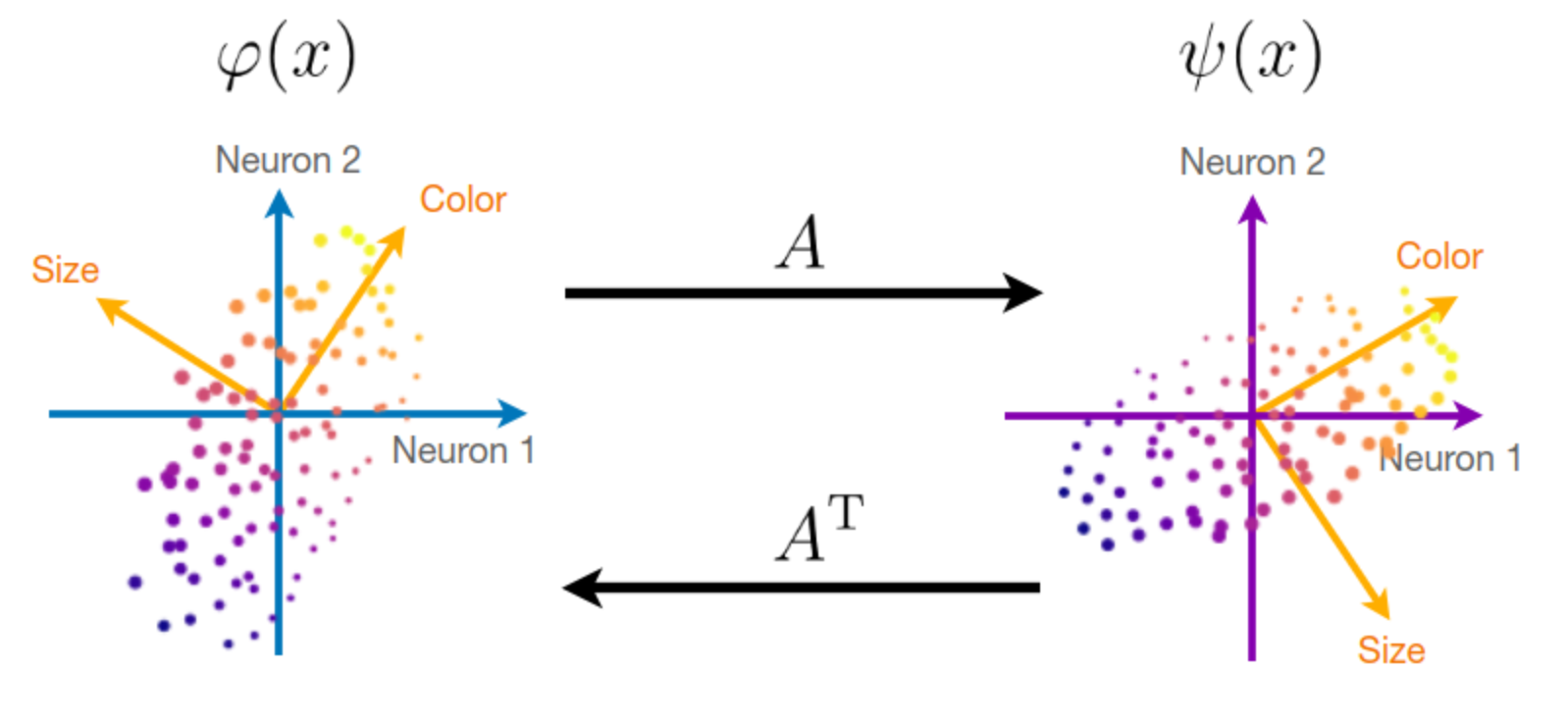
We wish to compute the best orthogonal alignment matrix A that aligns two representations \varphi(x) to \psi(x): \min_A \mathbb E_x[\|A\varphi(x) - \psi(x)\|^2] \quad\text{such that}\quad A^\top A = I_d

This is akin to a linear regression, but additionally imposes that A is orthogonal in order to preserve the geometry of the latent dimensions of the representations.

The optimal alignment A can be computed explicitly from an SVD of the cross-covariance matrix:

A = U V^\top \quad\text{with}\quad \mathbb E_x[\psi(x)\varphi(x)^\top] = U\Sigma V^\top

The magnitude of the singular values \Sigma indicate the amount of variance that is explained by the alignment A. Indeed, the unexplained variance (the residual error) can be written as: \mathbb E_x[\|A\varphi(x) - \psi(x)\|^2] = \mathbb E_x[\|\varphi(x)\|^2] + \mathbb E_x[\|\psi(x)\|^2] - 2 \,\mathrm{tr}\ \Sigma

To evaluate the effectiveness of the alignment procedure, we can thus compute an r^2 measure as the ratio between the explained variance and the total variance: r^2 = \frac{\mathrm{tr}\ \Sigma}{\sqrt{\mathbb E_x[\|\varphi(x)\|^2]}\sqrt{\mathbb E_x[\|\psi(x)\|^2]}}

Compare cross-covariance between model activations

model1, model2 = models
cross_covs = compute_activation_covariances(train_loader, layers, model1, model2)
# cross_covs is a list of activation covariances (C1, C2) for each layer.

# We also compute the self-covariance of both model activations as we will need it later.
model_layer_covs = [activation_covariances] + [
    compute_activation_covariances(train_loader, layers, models[1])
]

Compute alignments between models with an SVD, and evaluate alignment accuracy (fraction of explained variance)

aligns = []  # layer_idx -> alignment
for j in range(2):
    cross_cov = cross_covs[j]
    u, s, vh = torch.linalg.svd(cross_cov, full_matrices=False)

    explained_variance = torch.sum(s)
    total_variance = torch.sqrt(
        torch.trace(model_layer_covs[0][j]) * torch.trace(model_layer_covs[1][j])
    )
    r_squared = explained_variance / total_variance
    print(
        f"Layer {j + 1}: {100 * r_squared.item():.1f}% of variance explained by"
        " alignment"
    )
    # NOTE: r² should be computed on a test set to control for overfitting.

    align = u @ vh
    aligns.append(align)

Layer 1: 92.2% of variance explained by alignment
Layer 2: 87.5% of variance explained by alignment

We see that the alignment procedure is able to explain a good fraction of the variance of the representations.

Using aligned networks to compare activation eigenvectors

Let us now use the alignment matrix A to meaningfully compare activation eigenvectors.

Assume that we have an activation eigenvector u for the first network, and another activation eigenvector v for the second network, which may or may not encode the same latent dimension. How do we compare them? Because A\varphi(x) \approx \psi(x), we should compare Au with v.

We can then compare each eigenvector for the first network after alignment with each eigenvector for the second network by measuring the cosine of the angle between them. This is a matrix that we can visualize. In fact, this matrix computes the orthogonal change of basis from the (aligned) eigenvectors for the first network to the eigenvectors for the second network. If it is close to the identity, then the two sets of eigenvectors are almost the same. On the other hand, if the eigenvectors are really different, then no entry of this matrix will be close to unity.

Note that the eigenvectors of a matrix are determined up to a reverse in direction. This means that v and -v correspond to the same eigenvector. To this end, to compare two sets of eigenvectors, we look at the absolute values of the entries of the change of basis matrix.

Compare eigenvalues and eigenvectors of the activation covariances of both networks

fig, ax = plt.subplots(figsize=(9, 9), nrows=2, ncols=2)

for j in range(2):
    # Compute activations spectrum and eigenvectors for each model.
    activation_spectra = []
    activation_eigenvectors = []
    for layer_covs in model_layer_covs:
        cov = layer_covs[j]  # (C, C)
        eigenvalues, eigenvectors = torch.linalg.eigh(cov)
        # Sort in descending order and transpose.
        eigenvalues, eigenvectors = eigenvalues.flip(-1), eigenvectors.flip(-1)
        eigenvectors = eigenvectors.T  # (R, D)
        activation_spectra.append(eigenvalues)
        activation_eigenvectors.append(eigenvectors)

    # Compare activation spectra.
    plt.sca(ax[0][j])
    plt.title(f"Activation covariance eigenvalues (layer {j + 1})")
    for i, spectrum in enumerate(activation_spectra):
        y = spectrum.cpu().numpy()
        x = 1 + np.arange(len(y))
        plt.plot(
            x,
            y,
            color=["tab:green", "tab:purple"][i],
            linestyle=["solid", "dashed"][i],
            label=f"Network {i + 1}",
        )
    plt.yscale("log")
    plt.xscale("log")
    plt.xlabel("Rank")
    plt.ylabel("Eigenvalue")
    plt.legend(loc="upper right")

    # Compare activation eigenvectors after alignment.
    plt.sca(ax[1][j])
    stab = torch.abs(
        activation_eigenvectors[0] @ aligns[j] @ activation_eigenvectors[1].T
    )
    plt.imshow(stab.T.cpu().numpy()[:50, :50], cmap="cividis", vmin=0, vmax=1)
    plt.colorbar(shrink=0.75)
    plt.title(f"Comparison of activation eigenvectors (layer {j + 1})")
    plt.xlabel("Rank (network 1)")
    plt.ylabel("Rank (network 2)")
    ticks = np.asarray([1, 10, 20, 30, 40, 50])
    plt.xticks(ticks=ticks - 1, labels=[str(i) for i in ticks])
    plt.yticks(ticks=ticks - 1, labels=[str(i) for i in ticks])

plt.tight_layout()
plt.show()

Using aligned networks to compare weight eigenvectors

Similarly, suppose that u and v are now weight eigenvectors respectively for the first and second network. The weight eigenvector u applies on the representation \varphi(x), computing \langle u, \varphi(x) \rangle, while the weight eigenvector v applies on the the representation \psi(x), computing \langle v, \psi(x) \rangle. We then have

\langle u, \varphi(x) \rangle = \langle Au, A\varphi(x) \rangle \approx \langle Au, \psi(x) \rangle,

which again means that we should compare Au with v.

Compare eigenvalues and eigenvectors of the weight covariances of both networks

fig, ax = plt.subplots(figsize=(9, 9), nrows=2, ncols=2)

for j in range(2):
    # Compute weight spectrum and eigenvectors for each model.
    weight_spectra = []
    weight_eigenvectors = []
    for model in models:
        w = model[2 * j + 1].weight  # (N, D)
        u, s, vh = torch.linalg.svd(w, full_matrices=False)  # (N, R), (R,), (R, D)
        spectrum = s**2 / w.shape[0]
        weight_spectra.append(spectrum)
        weight_eigenvectors.append(vh)

    # Compare weights spectra.
    plt.sca(ax[0][j])
    plt.title(f"Weight covariance eigenvalues (layer {j + 1})")
    for i, spectrum in enumerate(weight_spectra):
        y = spectrum.cpu().numpy()
        x = 1 + np.arange(len(y))
        plt.plot(
            x,
            y,
            color=["tab:blue", "tab:orange"][i],
            linestyle=["solid", "dashed"][i],
            label=f"Network {i + 1}",
        )
    plt.yscale("log")
    plt.xlabel("Rank")
    plt.ylabel("Eigenvalue")
    plt.legend(loc="upper right")

    # Compute stability, with alignment if needed.
    if j > 0:
        stab = torch.abs(
            weight_eigenvectors[0] @ aligns[j - 1] @ weight_eigenvectors[1].T
        )  # (R, R)
    else:
        stab = torch.abs(weight_eigenvectors[0] @ weight_eigenvectors[1].T)  # (R, R)

    # Compare weight eigenvectors.
    plt.sca(ax[1][j])
    plt.imshow(stab.T.cpu().numpy()[:50, :50], cmap="cividis", vmin=0, vmax=1)
    plt.colorbar(shrink=0.75)
    plt.title(f"Comparison of weight eigenvectors (layer {j + 1})")
    plt.xlabel("Rank (network 1)")
    plt.ylabel("Rank (network 2)")
    ticks = np.asarray([1, 10, 20, 30, 40, 50])
    plt.xticks(ticks=ticks - 1, labels=[str(i) for i in ticks])
    plt.yticks(ticks=ticks - 1, labels=[str(i) for i in ticks])

plt.tight_layout()
plt.show()

After alignment, top eigenvectors strongly correlate across random initializations. We have seen that it is exactly these eigenvectors which matter for performance. The informative, learned weight and activation principal components are thus shared by both networks: they are universal!

Generating a new network without training

Do the covariances really encode all the information needed to explain the performance of the network?

We can check by generating new, random weights which have the same covariance as that of a trained network. This is done by drawing the weights of each neuron independently from a Gaussian distribution. Note: the generated network should be aligned to the original network in order to use the same weight covariances.

The generation is iterative, layer by layer:

Draw samples from \mathcal N\left(0, \frac{1}{n_1} W_1^\top W_1\right) for the weights W_1' of the first layer
Compute the alignment A_1 so that A_1 \sigma(W_1'x) \approx \sigma(W_1 x)
Draw samples from \mathcal N\left(0, \frac{1}{n_2} (W_2 A_1)^\top (W_2 A_1)\right) for the weights W_2' of the second layer
Compute the alignment A_2 so that A_2 \sigma(W_2' \sigma(W_1' x)) \approx \sigma(W_2 \sigma(W_1 x))
Set the classifier weights \theta' = \theta A_2

Sample a network using only covariance statistics

state_dict_keys = list(model.state_dict().keys())
print(f"Generating {state_dict_keys}")
reference_accuracy, generated_accuracy = generate_network(
    model, state_dict_keys, train_loader, val_loader
)
print(
    f"Accuracy after sampling: {generated_accuracy:.1f}% (accuracy after training:"
    f" {reference_accuracy:.1f}%)"
)

Generating ['1.weight', '3.weight', '5.weight']
Accuracy after sampling: 31.4% (accuracy after training: 42.7%)

Without any training, the generated network recovers a good fraction of the performance of the trained network. It implies that the covariances indeed encode most of the task-relevant information learned during training.

Extending the analysis to convolutional networks

We now consider a CNN, composed of two 5 \times 5 convolutional layers and a fully-connected classifier.

Initialize a convolutional neural network

channels = [1, 32, 64]
cnn_model = initialize_cnn_model(channels)
print(cnn_model)

Sequential(
  (0): Conv2d(1, 32, kernel_size=(5, 5), stride=(2, 2), bias=False)
  (1): ReLU()
  (2): Conv2d(32, 64, kernel_size=(5, 5), stride=(2, 2), bias=False)
  (3): ReLU()
  (4): Flatten(start_dim=1, end_dim=-1)
  (5): Linear(in_features=1600, out_features=10, bias=False)
)

Train the convolutional neural network

train_model(cnn_model, train_loader, val_loader, num_epochs=5)

Sequential(
  (0): Conv2d(1, 32, kernel_size=(5, 5), stride=(2, 2), bias=False)
  (1): ReLU()
  (2): Conv2d(32, 64, kernel_size=(5, 5), stride=(2, 2), bias=False)
  (3): ReLU()
  (4): Flatten(start_dim=1, end_dim=-1)
  (5): Linear(in_features=1600, out_features=10, bias=False)
)

In CNNs, the weights are no longer matrices but fourth-order tensors, of shape C_{\rm out} \times C_{\rm in} \times k_{\rm h} \times k_{\rm w}. This corresponds to n = C_{\rm out} neurons which compute linear projections over patches, of dimension d = C_{\rm in} \times k_{\rm h} \times k_{\rm w}.

We can thus reshape the weight tensor as a n \times d matrix W, and treat it as the weight matrix of a fully-connected network as above. We can thus compute the weight covariance as \frac{1}{n} W^\top W, which is a d \times d matrix.

weight = conv_layer.weight  # (C_out, C_in, k_h, k_w)
weight_flat = weight.reshape((weight.shape[0], -1))  # (C_out, C_in*k_h*k_w)
weight_cov = weight_flat.T @ weight_flat / weight_flat.shape[0]  # (C_in*k_h*k_w, C_in*k_h*k_w)

Similarly, the activations are no longer vectors but third-order tensors, of shape C \times H \times W. Rather than reshaping them as vectors, we will only compute covariances over channels and treat the spatial dimensions as additional samples. This means we will align the channels of two representations, but not their spatial dimensions. This is due to the translation-equivariance of CNNs, which preserve the spatial dimensions. The arbitrariness of the neural code is thus only along the channel dimension.

activations = (
    phi(x)  # (B, C, H, W)
    .permute(0, 2, 3, 1)  # (B, H, W, C)
    .flatten(start_dim=0, end_dim=2)  # (BHW, C)
)
activations_cov = activations.T @ activations / activations.shape[0]  # (C, C)

Sample a CNN using only covariance statistics

state_dict_keys = list(cnn_model.state_dict().keys())
reference_accuracy, generated_accuracy = generate_network(
    cnn_model, state_dict_keys, train_loader, val_loader
)
print(
    f"Accuracy after sampling: {generated_accuracy:.1f}% (accuracy after training:"
    f" {reference_accuracy:.1f}%)"
)

Accuracy after sampling: 36.0% (accuracy after training: 58.0%)

About two thirds of the performance of the trained network is captured in its covariances. Generating CNN weights with Gaussian distributions does not work as well because the spatial filters are not well-approximated by a Gaussian (due to selectivity in orientation and frequency).

The accuracy of the generation procedure can be improved by switching to an architecture which predefines the spatial filters, so that they are not learned nor randomly generated. This is achieved by learned scattering networks (Guth, Zarka, and Mallat 2021), which use wavelet spatial filters and learned weights along channels.

References

Guth, Florentin, Brice Ménard, Gaspar Rochette, and Stéphane Mallat. 2023. “A Rainbow in Deep Network Black Boxes.” arXiv. https://doi.org/10.48550/ARXIV.2305.18512.

Guth, Florentin, John Zarka, and Stéphane Mallat. 2021. “Phase Collapse in Neural Networks.” https://doi.org/10.48550/ARXIV.2110.05283.

Experimental setup

Dataset

Network architecture and training

Analyzing a trained network

Measuring the dimensionality of hidden representations

Measuring the dimensionality of neuron weights

Comparing neural networks

Aligning two networks together

Using aligned networks to compare activation eigenvectors

Using aligned networks to compare weight eigenvectors

Generating a new network without training

Extending the analysis to convolutional networks

Further reading

References